The Deepest Dive: Illustration Arbitrage in Participating Loans

Introduction

In previous Points articles, we explored how Fixed Participating and Variable Participating loans work. A key element to these loan types is the ability for arbitrage between the charge and crediting rates. Our examples attempted to provide real-life examples of what could happen when utilizing these types of loans. However, where these loans get commended, as well as notoriety, is how they illustrate within a Life Insurance illustration.

To understand how participating loan illustrations are run, and why they are designed the way they are, we will focus on two distinct areas: the regulatory environment, and the illustrated sales scenario.

The Regulatory Environment

The world of life insurance illustrations is bound by a series of regulations that determine the ways they can be run, and what disclosures must be stated within the output. The main regulatory framework is the Life Insurance Illustrations Model Regulation (#582), which came to be in 1997. However, since that time, product designs have innovated and changed in ways that weren’t originally accounted for. And with the advent of Indexed Universal Life (IUL) products, it became increasingly difficult for both consumers and advisors to compare “like” products. Not only did one have to view the variety of features and benefits, but even when illustrating at a maximum illustrated rate, using the same index with equal caps and floors, products could illustrate widely different results. In addition, as there were no standards in place, rates were seemingly up to the discretion of each carrier – they used varying lookback periods or newer market/indices that offered more advantageous returns, such as the Hang Seng, to help justify illustrated performance.

To address this, Actuarial Guideline XLIX (AG49) was adopted in 2015. It attempted to standardize life insurance illustrations by setting consistent limits on the credited and earned interest rates for policies with index-based interest, ensuring realistic and comparable projections across products. It also outlined clear guidelines for calculating these rates, required side-by-side illustrations with alternate scales, and mandated additional consumer disclosures. This approach aimed to eliminate overly optimistic and varied illustrations, enhancing transparency and consumer understanding. For a full understanding and deep dive of AG49 and its evolution, I recommend “Actuarial Guideline 49: A Look at the IUL Evolution Through Regulation & Product Design” researched and written by LifeTrends veteran, Sydney Presley.

For this post, we will focus on one specific element of AG49 – the arbitrage crediting spread on Participating Loans. Prior to AG49, companies were able to illustrate any spread they felt justified. For example, they could show a crediting rate of 8% and charge rate of 4%, creating a spread of 4%. AG49 addressed this initially by placing a 1% limit on the spread. This was lowered to .50% in a subsequent update. However, the language surrounding the spread is quite short.

If the illustration includes a loan, the illustrated Policy Loan Interest Credited Rate shall not exceed the illustrated Policy Loan Interest Rate by more than 50 basis points. For example, if the illustrated Policy Loan Interest Rate is 4.00%, the Policy Loan Interest Credited Rate shall not exceed 4.50%.

As we progress through this post, we will see how that sentence, and others, are interpreted by carriers.

Illustrated Sales Scenarios

The second key area is how the cases are designed for sales situations. For Indexed UL, a common sales scenario is a highly funded policy until retirement, premiums cease, and cash value distributions begin. This scenario is often called “Life Insurance Retirement Plan” or “LIRP”. The goal of this design is to provide supplemental retirement income while enjoying the inherent tax efficiencies of life insurance. The keyword is “supplemental” – most insurance compliance departments would have a conniption if it was advertised as THE retirement plan.

Within this structure there are many considerations: What type, and duration of distribution? How much cash value remains after the distribution phase? Death Benefit options? Etc… When LifeTrends launched our IUL benchmarks, carrier partners significantly contributed to the final design. Another colleague, Zaahirah Souri, succinctly outlined this in her article “Step Up your Set Up”. A summary is provided at the end of this post.

With an understanding of what goes into Max Dist benchmarking, let’s focus on the illustrated advantages associated with Participating Loans and how product design makes an impact.  

Table 1 below compares Annualized Maximum Distributions between Fixed Loans and Participating Loans benchmarks for a 45-year-old male, preferred, pay to retirement. As shown, for most carriers, Participating Loans perform stronger than Fixed Loans. This in itself is not surprising, as we mentioned with AG49, a .50% arbitrage is allowed and boosts higher cash value during the distribution years, thus increasing distribution amounts. What is interesting is the range of improvement. If everyone is limited to a .50% arbitrage you might logically conclude the benefit would be relatively the same, yet that’s not the case. Why? Product design and interpretations of AG49.

Table 1.

Current as of 7/10/24

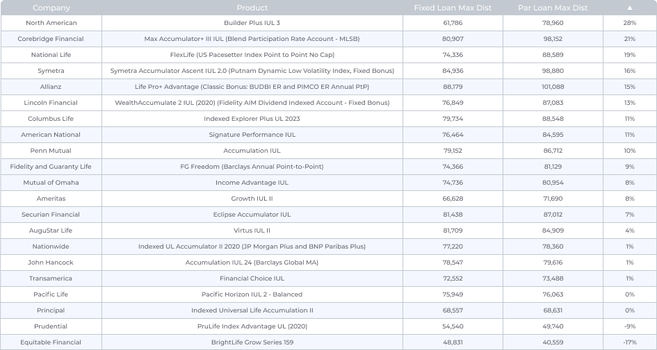
You’ll notice for Equitable Financial, their Fixed Loan illustrates better than the Participating Loan. Why? Our dear friend, Arbitrage!  However, this time it’s been flipped and a negative arbitrage is working against the client. The charge on their Participating Loan is 5.0% but their Maximum Illustrated rate is only 4.22%. Therefore, for every year there’s an outstanding loan balance, the client pays an effective rate of 0.78% on that debt. Equitable’s Fixed Loan has a 1% charge spread for the first 10 years and then becomes a wash loan. This means, with loans starting in year 20, Fixed Loans cost 0% while Participating Loans cost 0.78%. Prudential also performs better with Fixed Loans but it isn’t due to negative arbitrage. After digging in and doing some due diligence there does not appear to be an evident reason why.

The Bonus

One thing all companies in the benchmark, except Prudential and Mutual of Omaha, have in common is some form of Bonus on the policy. They’re in different forms and names such as; Account Value Enhancement, Persistency Credits, Bonuses, Index Credit, etc.. They operate differently from one another and have various levels of guarantees – some guaranteed for life at a guaranteed rate while others are a series of tests performed to determine if a bonus/credit should be applied. This post will not cover how they work or contrast, but rather focus on what they do to illustrated values.

Of the top ten products ranked by Max Dist, 7 also feature some of the largest bonuses in our benchmarks. In addition, while often offering a higher bonus, the year in which the bonus becomes eligible tends to be earlier. It logically follows that a higher bonus, starting earlier, will produce higher values than a lower bonus starting later.

Now that we’ve covered the impact a Bonus has in increasing Maximum Distributions, let’s discuss the assumptions in life insurance illustrations that generate this result.

1. Positive arbitrage occurs every year a loan is outstanding

As demonstrated in the benchmark outline, loans are taken “at retirement” (Age 65) for 20 years and no loan repayments are made. This fits with the sales scenario because the cushion, $10,000 CSV at Age 100, instructs the illustration to take the maximum amount of loans with enough remaining cash value to cover the outstanding loan debt. Therefore, there’s no need to pay them back!  Illustrated values prior to distribution for Fixed and Participating Loans are the same. Once distributions begin, the cash values will differ as the illustration must consider the $10,000 of Cash Value at age 100, which is where the difference between Fixed Loans and Par Loans occurs, that generate the higher returns.

Let’s assume a fixed wash loan – after 20 years, the outstanding loan balance should be equal to the loan collateral and will continue to grow equally until age 121. Often, the cash value either gets to, or near $10,000. Once it “bottoms out” it starts growing again as the accumulation value growth is a higher rate than the loan debt… every single year. If we switch to Participating Loans, during the 20 years of distribution, the accumulation value reduces less, due to the arbitrage adding value … every single year.

2. Bonuses are IN ADDITION to index crediting

It’s worth reviewing the language from the regulation for this section.

If the illustration includes a loan, the illustrated Policy Loan Interest Credited Rate shall not exceed the illustrated Policy Loan Interest Rate by more than 50 basis points. For example, if the illustrated Policy Loan Interest Rate is 4.00%, the Policy Loan Interest Credited Rate shall not exceed 4.50%.

The regulation defines the following:

• Policy Loan Interest Rate
  •  The current annual interest rate as defined in the policy that is charged on any Loan Balance. This does not include any other policy charges.

• Policy Loan Interest Credited Rate
  • The annualized interest rate credited that applies to the portion of the account value backing the Loan Balance:
    • For the portion of the account value in the Fixed Account that is backing the Loan Balance, the Policy Loan Interest Credited Rate is the applicable annual interest crediting rate.
    • For the portion of the account value in an Index Account that is backing the Loan Balance, the Policy Loan Interest Credited Rate is the Annual Rate of Indexed Credits, net of any applicable Supplemental Hedge Budget, for that account.

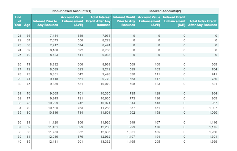
As you see, there is no statement about Bonuses . Therefore, some carriers take the Indexed Crediting from the Strategy selected (Policy Loan Interest Credited Rate), minus the stated charge rate (Policy Loan Interest Rate) to arrive at the 50 basis point (if they can). From here, the bonuses are applied to the loan collateral. There is nothing in the language that prevents this. Lincoln Financial clearly displays this in action on their WealthAccumulate IUL. In this example, we use the Fixed Account for our Strategy allocation and the Fidelity AIM Dividend Indexed Loan Account -Fixed Bonus, a Fixed Participating loan as defined by LifeTrends. This loan has a fixed guaranteed charge of 5.25% and the Fidelity AIM Dividend Indexed Loan Account -Fixed Bonus illustrates at 5.69%. If we take the 5.69% – 5.25% we get 0.44%. This is within the .50 spread outlined in the regulation so we’re good to credit at the full 5.69%. This is reflected in year 26, when a loan is taken for $10,000, the Interest credited is $569 ($10,000 x 5.69%). In the AVE column to its right, we clearly see the 1% Account Value Enhancement from the Fidelity AIM Dividend Indexed Loan Account -Fixed Bonus being applied and crediting $100. Combining the Indexed Interest Credit and the AVE, the total credit for that loan segment is $669 or a 6.69% return.

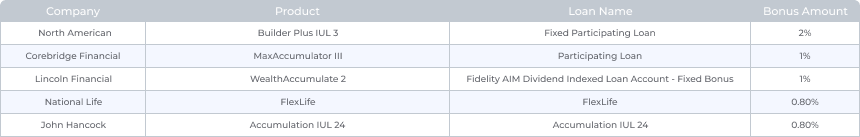
To be clear, not every carrier does it exactly like this. The interpretation of the Bonus applied after the indexed crediting is not universal. Also, not all Bonuses add to the loan collateral. Transamerica, American National, and Nationwide all have language that explicitly states their Bonus DOES NOT apply to loan collateral; conversely Allianz explicitly states it DOES. What is clear is that Bonuses on the loans themselves appear to be very effective in generating favorable arbitrage. With the exception of John Hancock, every company that offers a bonus on loan collateral sees a 15% or greater increase in Max Distributions over Fixed Loans. Additionally, 3 of the top 5 ranked by Max Dist offer this type of Bonus. The table below shows the products that are benchmarked that have a bonus that is tied directly to the loan itself (though, as mentioned above, other products might have the account bonus apply to loan collateral, such as Allianz). For details on product bonuses and indexed strategy bonuses, the recently launched Crediting section outlines that information.

Table 2.

Products with Loan Specific Bonuses

With the competitive landscape of Bonuses in participating loans covered I want to bring it back to assumptions.

Illustrations must use assumptions in order to generate values, and per the regulation, insurance companies illustrate current values at a rate no higher than the maximum determined in the regulation. Most illustrations will assume one rate for the life of the policy, as LifeTrends does on our benchmarks. This long-term assumption of a constant growth rate really unleashes the power of compounding interest. For example, most products have a maturity age of 121 and therefore illustrations tend to run to that age. 121 is quite old and obviously extremely unlikely to happen, so illustrated values at this age should not have any substantial importance. However, it’s a fun thought exercise to rationalize what the illustration shows. For example, let’s take the relatively straight-forward Columbus Life Indexed Explorer product. For the 45-year-old benchmark we’ve used throughout this post, the maximum distribution with Par Loans per year is $88,548. After the 20 years of supplemental retirement income, this client would have taken $1,770,960 tax free. Not a bad return for a $500,000 investment ($25,000 annual premiums over 20 years). But this policy is still in force and still has life to give, remember we assume the same growth every year. Let’s say the individual drinks 3 Dr. Peppers a day and makes it to age 121. They’d have $6,900,370 of Death Benefit and Surrender Value; combine that with the income benefit they received in retirement, they and/or their beneficiaries have returned over $8,500,000 in tax free money! That’s a 17x return on investment. If we did this exact same scenario, but utilize National Life FlexLife, which is a top 5 in Max Dist and features a Loan Specific Bonus, the total return is over $15,000,000, or a 31x return! The small difference in bonus amounts and indexed interest leads to dramatic differences due to the power of compounding.

The number of assumptions that go into illustrations, along with the amount of non-guaranteed elements that change at various intervals, make one thing clear… what actually happens in “reality” is ALWAYS going to be different than the illustration. That doesn’t mean it’s significantly worse or better, but it will absolutely be different. Here in lies the greatest challenge in attempting to provide consumers with an expectation of returns with non-guaranteed products. The current regulatory framework is doing its best, but it’s vagueness and the durations involved allow for small policy design adjustments to have large impacts on hypothetical values.

A curious piece of documentation was discovered in research for this post. It’s a draft of AG49 from 2019 that includes the following revision to the Policy Loans section

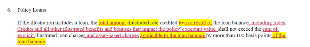
Let’s be blunt… if this version of the regulation had actually been adopted, this article would not exist, or at a minimum, be much shorter. This draft is much clearer on determining the final rate used for these loans. It’s not for LifeTrends to decide what’s more effective or right, but it’s interesting to imagine what current product design would look like with this language.

Conclusion

Life insurance illustrations are a key component of the sales process used for Indexed Universal Life. Regulations attempt to put carriers on a level playing field and to provide a “more realistic” set of expectations. Insurance companies have introduced product designs that are beneficial on their own, but also have the ability to improve illustrated values by a noticeable amount. One of these design enhancements we’re seeing increasingly adopted is a bonus applied to the loan collateral. In reality, and in illustrations, these bonuses help increase cash value, but it’s the assumptions of a life insurance illustration that really make them effective. And as always, it’s important for agents and clients alike to be informed and choose a product that fits their specific needs and appetite for risk.

This article is the conclusion of our deep dive into loans in the IUL space. Our first post started with the basics of loans, and we ended with the current product design landscape. You can look forward to more articles around loans in Whole Life, as well as a peek into recent trends within the Term space.

---

Maximum Distribution Illustration Set-Up